Image Style Transfer
What is Style Transfer?
Neural style transfer blends two images: the content of one (objects and their layout) and the style of another (colors, textures, brush strokes).
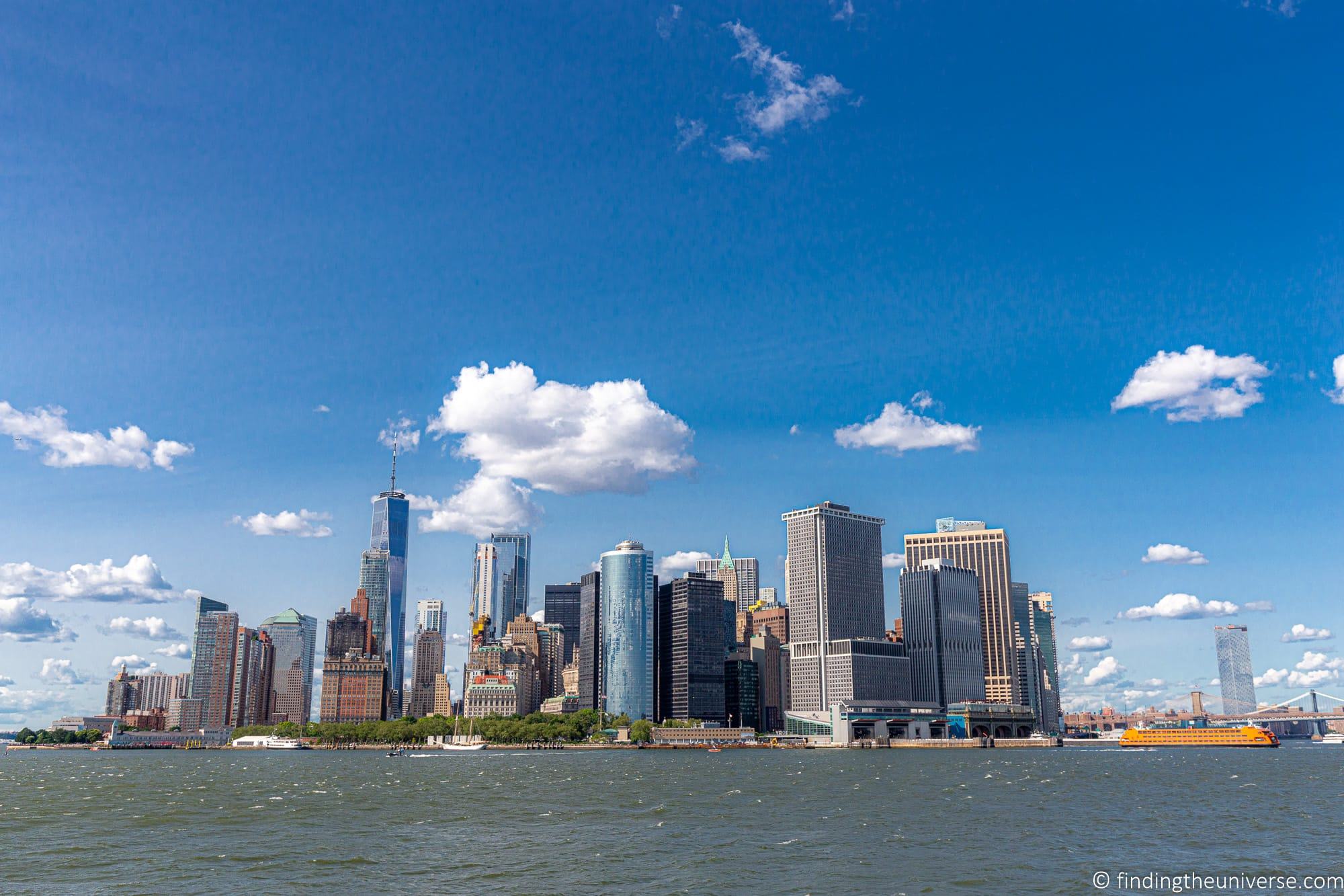
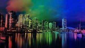
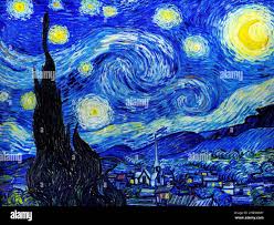
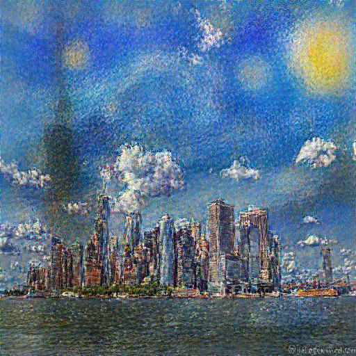
Think of it this way: take a photo of a city at night (content) and Van Gogh’s Starry Night (style). The goal is to produce a new image that keeps the city’s structure but paints it with Van Gogh’s swirling, vibrant style.
Why I Picked This Paper
I picked this paper because it’s not just about numbers and accuracy — it’s about turning algorithms into art. Style transfer felt like a great way to explore deep learning while creating something people can instantly connect with.
About the Paper
Image Style Transfer Using Convolutional Neural Networks (Gatys et al.) introduced a simple but powerful idea: use a pre-trained CNN (like VGG19) to separate content and style from images, then recombine them to create something entirely new.
At the core is the concept of deep image representations:
- Content representation: captures the structure and layout of objects in an image.
- Style representation: captures the textures, colors, and artistic patterns that define its “look.”
By defining losses for both and optimizing a new image, the method produces results that look like real paintings.
Content Representation
In a CNN, each layer extracts different levels of information:
- Early layers: detect edges and basic textures.
- Deeper layers: capture shapes, objects, and their arrangement.
For content, Gatys et al. take the feature maps from a deeper layer of VGG19. These maps summarize “what” is in the image (objects and layout) while ignoring pixel-level details.
The content loss is calculated by comparing the feature maps of the generated image to those of the original content image.
Style Representation
Style focuses on how the image looks — its brush strokes, color palettes, and repeated textures.
To measure style, the paper uses the Gram matrix of feature maps at multiple layers. The Gram matrix encodes correlations between features, acting like the image’s artistic fingerprint.
The style loss is calculated by comparing Gram matrices of the generated image and the style image.
Implementation: My Journey
When I started implementing this paper, I had one goal in mind: do everything from scratch. I didn’t want to simply import some ready-made library that spits out results. Instead, I wanted to truly understand how style transfer works — every function, every calculation, step by step.
At first, I chose NumPy + ONNX for this.
I downloaded the VGG19 model from the ONNX model zoo and wrote functions for:
- Running inference with ONNX Runtime
- Extracting intermediate outputs (feature maps)
- Preprocessing images into the right format
- Computing content loss, style loss, and total style loss in NumPy
This setup worked well for the forward pass. But the real challenge came when I tried to implement backpropagation.
To optimize the generated image, I needed gradients of the loss with respect to the image. That meant writing gradient functions for every single layer — convolution, ReLU, pooling, etc. Basically, I was re-inventing an entire deep learning framework.
I briefly looked at libraries like NumPy Autograd to handle the backprop part. But there was a big roadblock: ONNX Runtime only supports forward inference, not backward passes. NumPy Autograd couldn’t integrate with it. After a lot of research, I realized this path wasn’t practical.
So I made a key decision: switch to PyTorch.
- PyTorch already supports both forward inference and backpropagation.
- It automatically builds a computational graph, making optimization possible.
But — and this was important to me — I didn’t want to just rely on PyTorch for everything. My goal of learning from scratch remained the same. So I only used PyTorch for:
- Backpropagation (gradients + optimization)
And I still wrote everything else myself:
- Content loss function
- Style loss with Gram matrices
- Total style loss calculation
- Preprocessing and postprocessing functions
In the end, switching to PyTorch allowed me to finish the project while staying true to my original plan: build the main blocks myself instead of depending on heavy, pre-built solutions.
Building Blocks of the Project
1. Content Loss
The first block I implemented was Content Loss.
In a CNN like VGG19, each layer learns different patterns:
- Early layers → edges, colors, simple textures.
- Deeper layers → shapes, objects, and layouts.
For content representation, the paper uses a deeper layer (for example, conv4_2) of VGG19. This layer captures the “what” of the image — objects and their arrangement — while ignoring small pixel-level details.
The idea behind content loss is simple:
- Pass both the content image and the generated image through the CNN.
- Extract their feature maps at the chosen layer.
- Compute the squared difference between them.
Formula (from the paper):
$$ L_{\text{content}}(p, x, l) = \frac{1}{2} \sum_{i,j} (F^l_{ij} - P^l_{ij})^2 $$Where:
- Pl = feature maps of the content image at layer l
- Fl = feature maps of the generated image at layer l
- i = filter index
- j = position in the feature map
Intuitively: if the generated image’s features look like the content image’s features, the network preserves the original structure.
My Implementation in PyTorch:
def content_loss(ori, gen):
    return torch.sum((ori - gen) ** 2) / 2
Here:
ori → content feature map (from the content image).
gen → content feature map (from the generated/noise image).
The function simply calculates the squared difference. By minimizing this loss, the generated image learns to keep the layout and structure of the content image.
2. Style Loss
If content loss tells the network what to keep, then style loss tells it how the final image should look — its textures, strokes, and color patterns.
This is the artistic fingerprint of the style image. For example, whether it looks like Van Gogh’s brush strokes, watercolor splashes, or a sketch.
How do we capture style?
The paper uses the Gram Matrix of feature maps.
- Feature maps themselves show what is in an image.
- The Gram Matrix measures relationships between filters — how often patterns/textures appear together across the image.
This is why it captures style instead of object location.
Steps:
- Pass both the style image and the generated image through the CNN.
- Extract feature maps from multiple layers (because style exists at different abstraction levels).
- For each layer, compute the Gram Matrix.
- Compare the Gram Matrices of the style image vs. the generated image (using mean squared error).
Formula for style loss at one layer (from the paper):
$$ E_l = \frac{1}{4 \, N_l^2 \, M_l^2} \sum_{i,j} \left(G^l_{ij} - A^l_{ij}\right)^2 $$Where:
- Nl = number of filters in layer l
- Ml = height × width of the feature map
- Gl = Gram matrix of the generated image
- Al = Gram matrix of the style image
The total style loss is the weighted sum across all chosen layers:
$$ L_{\text{style}}(a, x) = \sum_{l} w_l \, E_l $$My Implementation
def gramm_matrix(arr):
    B, C, H, W = arr.size()
    arr = arr.reshape(C, H * W)
    return arr @ arr.t()

def style_loss(ori, gen):
    B, C, H, W = ori.size()
    ori = gramm_matrix(ori)
    gen = gramm_matrix(gen)
    M = H * W
    return torch.sum((ori - gen) ** 2) / (4 * (C ** 2) * (M ** 2))

def total_style_loss(w, E):
    ans = 0
    for i in range(len(w)):
    ans += w[i] * E[i]
    return ans
gramm_matrix → creates the style “fingerprint” of an image.
style_loss → compares style between generated and style image for one layer.
total_style_loss → combines losses across multiple chosen layers with weights.
By minimizing this loss, the generated image gradually learns to paint like the style image, while still holding the content from the original.
3. Style Transfer: Combining Content and Style
At this point, we have two separate ideas:
- Content loss → makes sure the output image keeps the structure of the content image.
- Style loss → makes sure the output image looks like it was “painted” in the style image.
But what we really want is both at the same time.
The Core Idea
We start with a random image (often white noise) and update it so that:
- Its content features match the content image.
- Its style features match the style image.
This is achieved by minimizing a total loss function:
$$ L_{\text{total}}(p, a, x) = \alpha \, L_{\text{content}}(p, x) + \beta \, L_{\text{style}}(a, x) $$Where:
- p = content image
- a = style image
- x = generated image
- α = weight for content loss (how much structure is preserved)
- β = weight for style loss (how much style is applied)
👉 The ratio of α (alpha) to β (beta) is crucial:
- High α, low β → output looks more like the content image.
- Low α, high β → output looks more like the style image.
- Balanced α, β → a proper fusion of both.
My Implementation
def total_loss(content_representation, styles_representation, noise_img, model):
    wl = [0.2, 0.2, 0.2, 0.2, 0.2] # weights for style layers
    alpha = 1
    beta = 1e4

    noise_content, noise_style = model(noise_img)

    loss_content = content_loss(content_representation[0], noise_content[0])
    loss_style = []
    for i in range(len(noise_style)):
    loss_style.append(style_loss(styles_representation[i], noise_style[i]))

    loss_style_total = total_style_loss(wl, loss_style)

    loss_total = (alpha * loss_content) + (beta * loss_style_total)
    return loss_total
Why this matters
This single function is the heart of the project — it decides how much “content” vs. how much “style” flows into the final output. By just tuning alpha and beta, we can make the result look more realistic, more artistic, or somewhere in between.
4. Optimization Loop
Once we have the total loss function (content + style), the next step is to actually optimize the generated image so that its pixels evolve into something meaningful.
The Role of Optimization
We start with a noisy image (random pixels). At every iteration, we slightly adjust the pixels so that:
- The content loss gets smaller (the structure looks more like the content image).
- The style loss gets smaller (the textures look more like the style image).
Over many iterations, the noisy image gradually transforms into the final stylized output.
Why L-BFGS?
I choose the L-BFGS optimizer (Limited-memory Broyden–Fletcher–Goldfarb–Shanno). It’s a quasi-Newton method that’s very efficient for this type of optimization because:
- It works well with problems where the number of parameters is huge (like optimizing every pixel of an image).
- It requires less memory than standard BFGS.
- It converges quickly, often in fewer iterations compared to simple gradient descent.
In simpler terms → L-BFGS is like a “smart gradient descent” that remembers past steps to update the image more efficiently.
My Implementation
def optimize_loop(noise_img, content_representation, styles_representation, model, iter):
    noise_img = noise_img.clone().detach().contiguous().requires_grad_(True)
    optimizer = torch.optim.LBFGS([noise_img])

    for i in range(iter):
    def closure():
    optimizer.zero_grad()
    loss = total_loss(content_representation, styles_representation, noise_img, model)
    loss.backward()
    print(f"Iteration {i}, Loss={loss.item():.2f}")
    return loss
    optimizer.step(closure)
    return noise_img
Key Point
Here, PyTorch automatically calculates the gradients of the total loss with respect to each pixel in the noisy image. The optimizer then updates those pixels, step by step, until the output image reflects both the content and the style.
5. Preprocessing and Postprocessing
Before feeding images into the model, I had to make sure they were in the format VGG19 expects.
Preprocessing
- Used ImageNet mean and standard deviation for normalization:
- Converted images into a 4D tensor (batch_size × channels × height × width).
- Instead of resizing to 224×224 (default for classification), I used 512×512 to preserve richer details.
- Avoided issues with fully connected layers by stopping the model before FC layers and only using convolutional layers for feature extraction.
Postprocessing
After optimization, the output is still a PyTorch tensor (with normalization applied). To convert it back into an actual image:
- Denormalize it (reverse the mean and std).
- Clamp values into the [0, 1] range.
- Use PIL to save the tensor as an image (.jpg or .png).
Why This Matters
Without proper preprocessing, the model won’t extract the right features — colors and textures may look off. And without postprocessing, the optimized tensor is just numbers — not something you can actually view or share.
The Tricky Part: System Resources
One of the biggest challenges I faced was computation time.
On my local system (CPU), running just 50 iterations took almost 30 minutes, and the results were still not great.
To get decent results, you usually need 300–500 iterations. On my machine, that would have taken hours.
The Solution
- Google Colab (GPU T4)
- NVIDIA RTX 3080
With these GPUs, the same 300–500 iterations took just 5–6 minutes — a huge improvement compared to my CPU runs.
This was a big learning point: style transfer is beautiful, but also very resource hungry.
Results
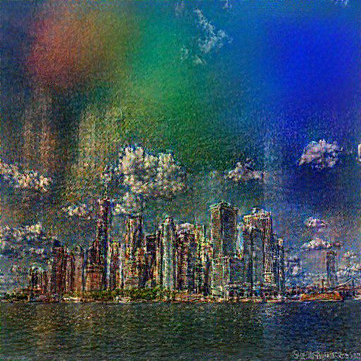
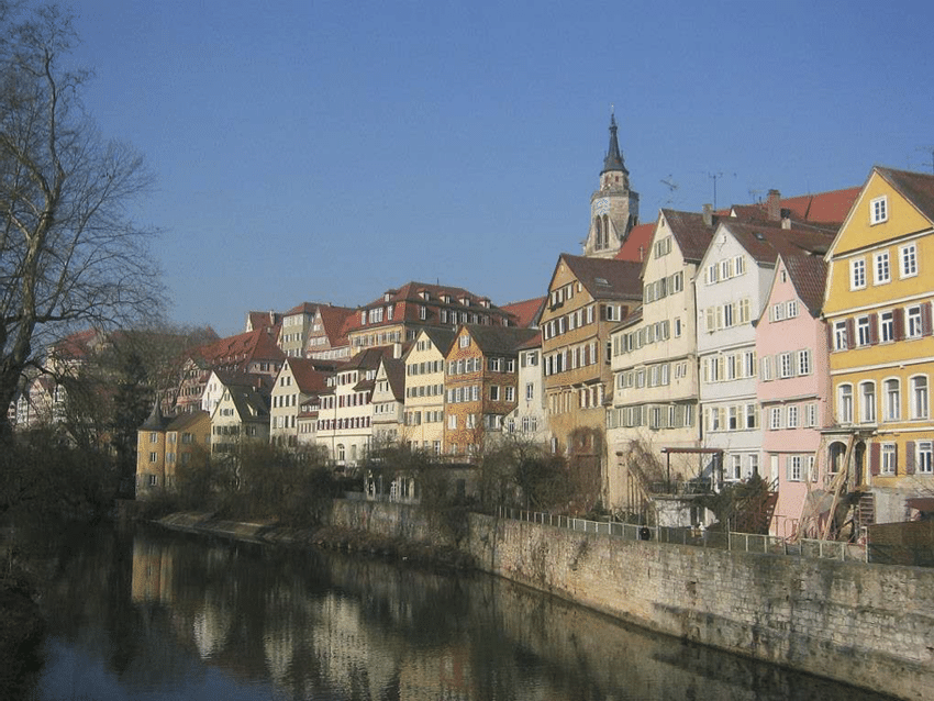
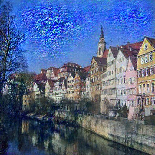
Here are some examples from my implementation (content + style → output):
Below is a few results showing how the content image and style image combine to create the final stylized output.
 +
+
 =
=
 +
+
 =
=
 +
=
+
=
Future Work
While the current implementation works, there are many ways to extend it:
- Reduce training time — experiment with faster optimization methods or smaller networks.
- Multiple styles — blend more than one style image into a single output.
- Deployment — build a small GUI or web app where users can upload content/style images and get outputs instantly.
Project Repository
You can explore the full code here: